


Beyond numbers: Unlocking customer insights with demand models


The amount of data companies gather is staggering and is only going to grow further. That fact, together with increased computational capabilities, already allows companies to build more accurate models, update their pricing more quickly, etc. This fact was already highlighted in McKinsey’s report in 20211 and most of those forecasts are slowly being realized.
However, what is probably not discussed enough is that it also allows insurance companies to better understand their customers and their rationale behind decisions whether to buy or decline a policy quote. Here comes demand modelling – a method of unlocking customer insights and improving insurance pricing processes!
What are demand models?
A simple definition of demand models is provided by IFOA’s Demand modelling working party2:
A demand model is a model of customer behaviour, which seeks to predict future behaviour based on an analysis of past experience. In particular, it looks at the propensity of a customer to purchase a product (insurance, for example), and how the propensity changes based on the price of the product.
The last sentence provides a crucial detail on their importance for insurance companies and a simplified way of thinking about demand models – they help companies predict how likely a customer is to buy a policy at a given price.
What that means is assuming a particular risk tolerance and uncertainty accepted by the company, they could try offering such premium level that maximizes the profit margin from a particular policy or even all aggregated policies. This aspect will be further explored in our upcoming article on Price Optimisation; however, it's essential to highlight its significance here. Therefore, this article will focus on modelling individual customer demand, their price elasticity, and state-of-the-art techniques to unlock this more individual and personalized view.
Importance of price elasticity
Elasticity is and has been a term widely used in economics studies for many years now, especially microeconomics which tends to look at markets and their participants in a greater detail.
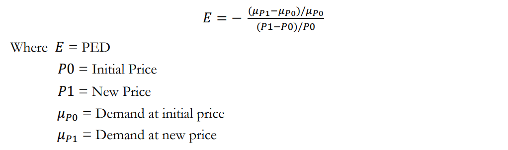
Price elasticity of demand (PED) was first defined by Alfred Marchall in Principles of Economic3 in 1890 and describes a change in demand for a given change in price. The value obtained tries to measure how sensitive a customer is to a (marginal) change in price, e.g., an insurance product. We say that customers are elastic, where their PED is high (greater than 1) and inelastic where the PED is low (lower than 1). This is summarised below:
To better understand that let’s consider an example:
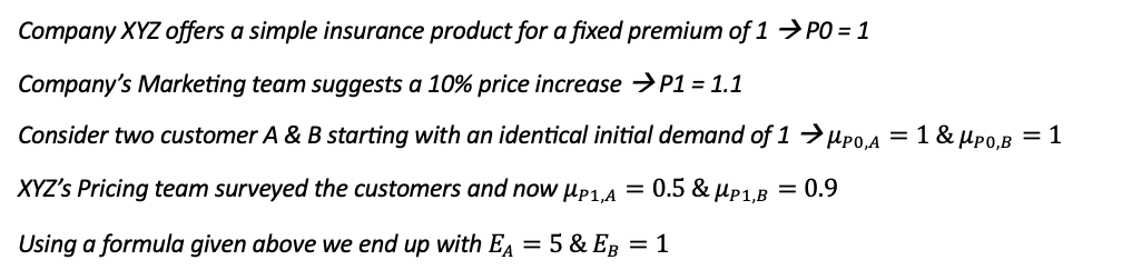
Respective values of EA & EB suggest that customer A is significantly more elastic than customer B – increase in product price results in a significant change in demand for the customer A, whereas for customer B it is perfectly inline with a change in product Price.
Having sufficient knowledge of the PED for goods allows someone selling that good (e.g., insurance company selling insurance product) to make informed decisions about their pricing strategies. This metric provides sellers with information about consumer pricing sensitivity.
Are demand models just a recent trend?
Actually, no! In fact, demand models have been around for decades; however, lack of computational power was often a limiting factor for many companies. However, in the era of big data and artificial intelligence, insurers are harnessing the power of advanced algorithms to refine their pricing models. Therefore, actuaries are now able to utilize linear and non-linear techniques to better capture different patterns of customer behaviours.
Data & modelling considerations
Data
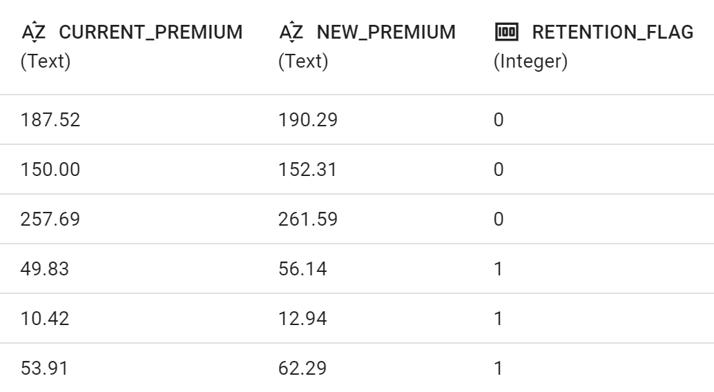
The most common approach to demand models is to create a classification model in which predictions would act as a probability of a take up of the policy, e.g., renewal policy. Therefore, the dataset would contain two variables indicating premium level (e.g. CURRENT_PREMIUM & NEW_PREMIUM or CURRENT_PREMIUM & RENEWAL_FACTOR) as well as a response variable in a form of a conversion flag attaining a value of 0 if the offered policy was rejected or 1 if accepted by the prospect.
Insurance companies often struggle with gathering the necessary data for modelling demand. There are neither clear guidance nor golden rules with respect to creating a questionnaire or agreeing on fo how long the quote remains open before being considered rejected, etc.
Some examples of gathering data for the purpose of Demand models have been described in our previous blog post4
Generalised Linear (or Additive) Model Approach
In a traditional approach, an actuary would try to fit a GLM to model the PED of the customers in the portfolio. This approach requires the following decisions to be made:
- Choice of target distribution
- Choice of a link function
- Model structure
- Final parameters
Target distribution
Since the model response variable attains values of 0 & 1, the binomial distribution seems to be a natural choice.
Link function
In order to properly choose a link function, actuaries have to consider that requirement of the link function is to transform the resulting coefficients from the structural design into a result that is consistent with the laws of probability as well as ensure the fitted response falls between 0 and 1.
Here two natural choices are then:
- Logit (logistic) function
- Probit (normal) function
Model structure
Since there are multiple insurance companies on the market, they often want to scrutinise PED taking into consideration its pricing strategies relative to their competitors, hence a variable in a form of
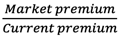
is very common5. The example of Market_premium calculation would be to average out quotes for customer with similar characteristics offered by N biggest competitors of the company or to use the market’s lowest offering for a customer with quoted characteristics. Then the model function attains the following form:
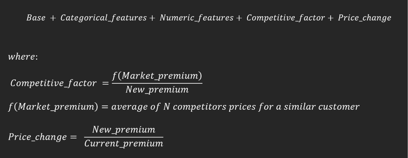
The last component quantifies a rate of change of the premiums – a relative price increase or decrease offered by a company.
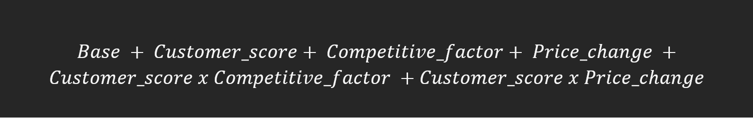
Now, if a new variable called Customer_score is introduced which is dependent on the categorical and numeric features of the prospects so that:

The model form can be written as:

This model structure allows to look separately at the impact of price-related and customer characteristics (Customer_score). The final step is to include interaction terms between those two types of variables leading to:
Choosing the parameters
In this final step, a pricing analyst or actuary would run several GLMs, compare them with statistical tests, apply some expert judgement and select the best model for the purpose. To better understand how to select the best model, please do not hesitate to check out one of our previous articles6.
Modern ML methods
Alternatively, the actuary could have run a modern Machine Learning model for the classification problem. The most obvious choice here would be one of the tree-based estimators such as: Decision Tree, Random Forest or Gradient Boosting Machine.
The main advantage is that Modern ML methods (especially GBM) can pick up interactions automatically which is a massive modelling advantage. However, as it is a case with many important pricing topics, most of the advantages that Modern ML could provide have already been covered by one of our previous blog posts7.
A more direct demand models advantage from using modern ML is that it allows users to gain accuracy in a relatively fast way which could be extremely beneficial in a scenario when an insurance company struggles with resources. On the other hand, some of the methods do not allow to constrain monotonicity in terms of price/price elasticity relationship.
Constraints
Demand models built on quotations that were not subject to price tests are usually not very accurate. Most demand models are only decent at predicting in the range of our price tests, e.g., if we did price tests varying from +-10%, our model might not be great for the +-20% range.
Another point is that the market environment is rapidly changing and we demand models become much quicker outdated than risk models, so they need to be recalculated often, e.g., on a monthly basis.
The demand model objective function is often required to be monotonic – there should be no bumps along the smooth curve. It originates from the assumption the reasonable consumer won't buy the product at a higher price when has an opportunity to buy cheaper.
In modern times, pricing tools can implement the monotonicity constraint with a simple toggle. However, behind the scenes, it is a very complex mathematical theory standing behind those reasons. To better understand the criteria for monotonicity of demand functions, the author kindly suggests referring to Criteria for Monotonicity of Demand Functions8.

How to use demand models
Utilizing demand models effectively involves a strategic approach that can be encapsulated into three primary methods: manual scenario analysis, customer segmentation and price optimization.
Manual Scenario Analysis
The first avenue of employing demand models is through manual scenario analysis. This method provides insights into how key performance indicators (KPIs) such as written premium and loss ratio would be affected by alterations in premiums.
By increasing or decreasing premiums, businesses can estimate the potential impact on sales and various written KPIs. This process allows for a granular understanding of the intricate relationship between pricing changes and overall business performance.
Customer Segment Analysis
A second pivotal use of demand models lies in understanding the dynamics of growth within different segments. These models offer a lens through which businesses can identify the specific areas where growth is occurring and, conversely, where it is diminishing.
By identifying these trends, organizations can tailor their strategies to capitalize on thriving segments while mitigating challenges in less buoyant areas. This segmentation-based approach facilitates a more targeted and efficient allocation of resources, fostering a more agile and responsive business strategy.
(Manual/Automated) Price Optimization
Lastly, demand models play a crucial role in price optimization, whether executed manually or through automated processes. The models aid businesses in determining the most optimal pricing strategies, considering factors such as market demand, competitor pricing, and internal cost structures.
This dual approach, whether manual or automated, ensures that businesses can adapt their pricing strategies dynamically to align with market fluctuations and internal considerations, thereby maximizing profitability and competitiveness. As already indicated, this topic will be the main theme of our upcoming article.
Conclusion
It is evident that the industry is undergoing a significant transformation. Embracing innovative technologies and ethical practices, insurers are not only meeting the evolving needs of their customers but also reshaping the future landscape of insurance.
Understanding the delicate balance between demand and conversion is not just a necessity for insurers but a testament to their commitment to providing more personalised and tailored insurance solutions in a rapidly changing world.
References
- Insurance 2030—The impact of AI on the future of insurance - https://www.mckinsey.com/industries/financial-services/our-insights/insurance-2030-the-impact-of-ai-on-the-future-of-insurance
- IFOA’s Demand modelling working party https://www.actuaries.org.uk/system/files/documents/pdf/demandmodellingworkingpartyfullreport.pdf
- Principles of Economics: https://eet.pixel-online.org/files/etranslation/original/Marshall,%20Principles%20of%20Economics.pdf
- The quest for the Perfect Price – price tests in insurance pricing https://www.quantee.ai/resources/the-quest-for-the-perfect-price-price-tests-in-insurance-pricing
- Beyond the Cost Model: Understanding Price Elasticity and Its Applications: https://www.casact.org/sites/default/files/database/forum_13spforum_guven_mcphail.pdf
- How to build the best GLM/GAM risk models? https://www.quantee.ai/resources/how-to-build-the-best-glm-gam-risk-models
- The great compromise: Balancing Pricing Transparency and Accuracy https://www.quantee.ai/resources/the-great-compromise-balancing-pricing-transparency-and-accuracy
- Criteria for Monotonicity of Demand Functions - 1978, Polterovich, Victor and Mityushin, Leonid - https://mpra.ub.uni-muenchen.de/20097/1/MPRA_paper_20097.pdf
%2520(2).png)


