Geography modelling in insurance pricing

.avif)
Geography modelling is one of the most important ingredients when it comes to P&C insurance pricing, particularly in motor and property insurance. It enables insurers to incorporate spatial patterns into their risk and demand models, ensuring premiums reflect the varying risk levels and behaviours across different geographic locations and making sure that modelled effects are properly smoothed.
I have never met a single personal lines pricing actuary who claimed that including geography information and applying geographic smoothing into their pricing process is not important.
From this post, you will learn what are the most common approaches to geography modelling together with their pros/cons.
Data considerations
There is often a temptation to use as much geographic data as possible, including data from third-party sources. While this can be valuable, pricing actuaries should avoid redundancy and instead focus on obtaining granular and fair data.
For example, when modelling motor coverage risk, you might consider both REGION and POSTCODE data. However, POSTCODE often captures the same information as REGION, so using both could be excessive and lead to overfitting in GLM/GAM models.
It’s better to seek third-party data that adds new insights, for instance social information or NatCat risks (check for instance Skyblue software). However, be careful with geo-social factors, as their improper use can lead to unintended discrimination in your models.
Available methods
Two methods within the insurance pricing community stand out for their utility and precision:
- 2D thin-plate splines
- Credibility-weighted residuals smoothing
Both of these methods are spatial smoothing methods i.e. they take into account geographical information to improve the precision of modelling + they make sure that the modelled target variable (for instance risk) doesn’t depend only on the policyholder area, but also on surrounding areas.
Both of these methods are applied to make GLM/GAM risk and demand models more precise, and both rely on some form of distance/neighbourhood relation between values of regional variable (e.g. postcode or other less granular like state or county).
Now let’s explore details of each method.
2D thin-plate splines
Algorithm
In 2D thin plate splines, we assign coordinates to a regional variable i.e. latitude and longitude and apply an interpolation procedure to a two-dimensional surface generated by those two coordinates.
The algorithm minimizes a function that balances two objectives:
- Goodness of fit: Ensures the spline surface passes close to the data points.
- Smoothness: Penalizes overly complex surfaces, preventing overfitting.
The steps to apply the algorithm are as follows (please note that the real implementation has more caveats, for more info look in [1]):
- Define knots that will be generated over latitude and longitude
- Generate thin-plate spline basis by calculating distances between data and knots as well as generating polynomial basis T i.e. X_basis = [Distance matrix; T]
- Generate penalty matrix P on calculated knots which will serve as L2 penalty matrix and apply scale parameter i.e. scale * P
- Estimate GLM/GAM model plugging thin-plate spline basis to explanatory variables and penalty matrix scale * P to overall L2 regularization matrix.

Advantages
- Only geo-coordinates are required
- Can be implemented in one go during GLM/GAM fitting to speed up pricing updates and scenario testing
- Captures non-linear relationships between geographic variables and target variable effectively
Disadvantages
- Doesn't perform well in isolated regions, such as islands
- Only advanced software has proper implementation including working for large datasets
Credibility-weighted residuals smoothing
Algorithm
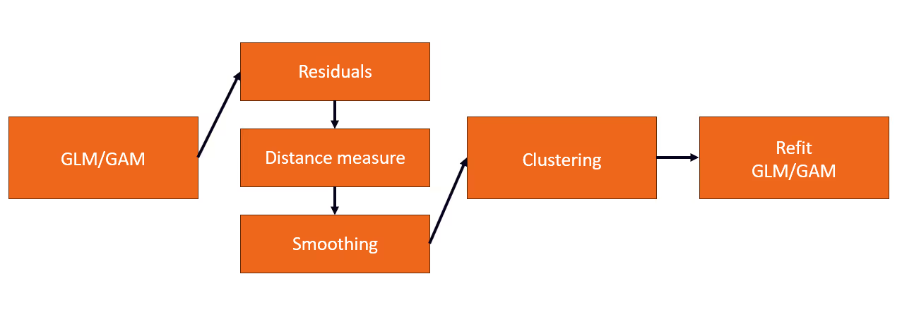
Credibility-weighted residual smoothing combines spatial smoothing techniques with actuarial credibility theory. The objective is to explain the residuals of GLM/GAM models with geographical information and smooth out the results.
Let’s look at the steps required:

- We build the best GLM/GAM model without geographical variables
- Smoothing
a) We calculate residuals 𝑟𝑝 by aggregating observed values and predictions by regional variable (e.g. postcode) and weighting them with exposure
b) We calculate distance measure 𝑑 (either distance-based from coordinates or adjacency-based from neighbours matrix)
c) We smooth residuals by applying a credibility-weighted smoothing function:

- Apply clustering on smoothed residuals to create a regional mapping
- Inject the regional mapping into the GLM/GAM model and refit

Advantages
- Effective on borders and isolated regions (islands).
- Mathematically and programmatically, it is easier to implement than 2D thin-plate splines.
Disadvantages
- Involves substantial manual work on distance matrix, residuals and refitting.
- Requires careful tuning of appropriate parameters for distance calculation and clustering.
- The need to apply additional extrapolation for postcodes not seen in training data in contrast to 2D thin plate splines which work on continuous coordinates.
Conclusions
In summary, we presented the two most popular methods for geography modelling and smoothing in the insurance community. The decision between these two methods is subjective and should be based on the results of your use cases.
If you’d be interested in more details about the implementation of these algorithms on real datasets, sharing your thoughts or discussing your current challenges please contact me at: dawid.kopczyk@quantee.ai.
References:
[1] Simon N. Wood, Generalized Additive Models An Introduction with R, Texts in Statistical Science, CRC Press, Second Edition.
%2520(2).avif)


