GLMs - Understanding their limitations in insurance pricing


When we start working in Pricing, the first thing most analysts want to do is jump right into modelling. Since GLMs are the most common approach and the one most of us learn first, that is usually where we begin.
If you were like me at the start, you probably went all in, testing different variables, tweaking transformations, adjusting categories, and trying all kinds of tricks—splines, logarithmic transformations, even finding interactions between two or three variables!
But sometimes, we get so focused on the model that we forget to take a step back. The truth is, GLMs have their limitations too. In this blog post, we’ll go over a few of them. Of course, each one could have its own dedicated post, but for now, let’s keep it simple!
In this post, we’ll discuss two key limitations of GLMs that stem from assumptions we make about them by default, which are not always correct:
- GLMs rely on the assumption that the data has full credibility
- GLMs rely on the assumption that the randomness of outcomes is uncorrelated.
1. GLMs rely on the assumption that the data has full credibility.
GLMs work under the assumption that all data has full credibility—meaning that estimates are treated as fully reliable, even when the available data is limited.
Let’s break this down with a simple example:
Imagine we’re building a pricing model for auto insurance in Mexico, aiming to estimate the severity of claims (the average cost per claim) across different cities. To keep things simple, we use a basic model where the only predictor is the city. The GLM will then estimate the expected average severity for each location. Here’s our dataset:
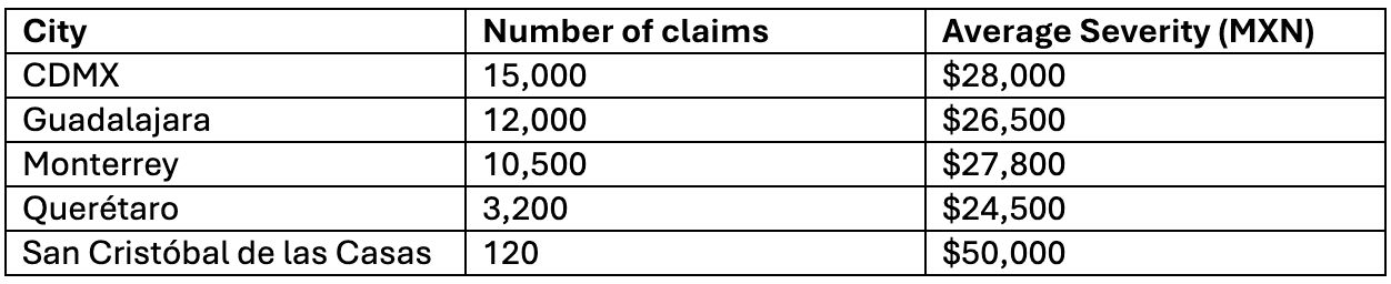
Our null model, in this case, will calculate the average severity for each city and assume it as correct. For San Cristóbal de las Casas, the model will take the expected severity of all claims as $50,000.
Here is the problem: In CDMX, Guadalajara, and Monterrey, we have thousands of claims, so the estimate is much more credible. In San Cristóbal de las Casas, we only have 120 cases, meaning that a single high-cost claim could have inflated the average significantly. The GLM doesn’t adjust for this automatically—it simply assigns the same credibility to all data, regardless of the sample size. That’s why the expert judgment of an actuary is crucial in supervising the model.
So... What now? What can we do about it? Are we done? Should we just give up on our model?
Okay, it's alright, don’t panic! With a bit of expert judgment and some actuarial tricks, we can fix this and get better results.
One Possible Solution: Bühlmann Credibility
One way to address this issue is by applying Bühlmann Credibility:
𝑆𝑒𝑣𝑖=𝑍⋅𝑋𝑖+(1−𝑍)⋅𝜇
Where:
𝑆𝑒𝑣𝑖: Adjusted severity for each city
𝑋𝑖: Observed severity for the city
𝜇: Expected severity of the overall group
𝑍: Credibility factor (determines how much weight is given to individual data vs. the group)
While 𝑍 can be calculated analytically, we won’t focus on that here. Instead, let’s focus on the concept:
- If a city has many claims, the estimate relies more on its own claim experience (higher 𝑍 )
- If a city has few claims, its estimate is adjusted more towards the overall average (lower 𝑍)
Applying Credibility to our example:
For San Cristóbal, since we have very few claims, let’s assume a credibility factor of 𝑍 0.2 for the sake of example:
𝑆𝑒𝑣(𝑆𝑎𝑛𝐶𝑟𝑖𝑠𝑡𝑜𝑏𝑎𝑙)=0.2×50,000+0.8×27,000=31,600
This smooths the estimate, preventing us from over-relying on small sample sizes.
Other Ways to Improve Estimates
There are other statistical methods that help adjust for low credibility data, including:
- GLMMs (Generalized Linear Mixed Models) → These allow cities with fewer data points to follow the overall trend rather than making extreme estimations.
- Regularization techniques (Elastic Net, Ridge Regression, etc.) → These penalize extreme estimates when data is scarce.
However, these methods go beyond the scope of this post. The key takeaway is that simple GLMs assume all data is fully credible, but in reality, expert knowledge is crucial to avoid misleading results.
2. GLMs rely on the assumption that the randomness of outcomes is uncorrelated.
What does it mean?
This essentially means that the model treats each record in the dataset as if it exists in its own little bubble, without recognizing any inherent relationships between them. It’s like assuming that every driver on the road makes decisions independently—when in reality, one reckless driver cutting people off can trigger a chain reaction of honking, sudden braking, and chaos.
However, this is only partly true. GLMs assume that each factor’s contribution to the prediction is independent of the others, which is why we need to explicitly add interaction terms to capture how one factor influences another. At the same time, the model is trained on the entire dataset, optimizing its coefficients (betas) to minimize differences between predictions and actual data—so while it doesn’t account for interactions on its own, it does pick up on overall patterns in the data.
In the same way, many data points in real life are connected and influence each other, even if the model doesn’t see it that way at all!
This means that the model treats each record in the dataset as if it exists in isolation, without recognizing any connections between them. It’s like assuming that every driver on the road makes decisions independently—when in reality, one reckless driver cutting people off can cause a chain reaction of honking, sudden braking, and chaos.
But this assumption isn’t always true. GLMs assume that each predictor affects the outcome independently unless we explicitly add interaction terms to capture how variables influence each other. At the same time, the model is trained on the entire dataset, adjusting its coefficients (betas) to minimize the difference between predictions and actual results. So while GLMs don’t automatically account for interactions, they can still pick up on general patterns in the data.
In real life, many data points are connected and influence each other, even if the model doesn’t recognize it directly. That’s why actuaries play a key role in supervising the model, identifying hidden relationships, and ensuring the predictions make sense.
Why is this a problem?
If there are groups of records that are actually related, but the model doesn’t account for it, it can lead to errors. Let’s look at a couple of examples to understand this better:
A) Auto Policy Renewals: A hidden trap for GLMs!
Imagine we’re analyzing auto insurance data, tracking customers who have renewed their policies over several years:
- Each year appears as a separate row in the dataset
- A driver who had an accident in Year 1 is likely to have similar driving behavior in the following years.
- But... the GLM treats each year as if it were a completely different driver!
Because of this, the model doesn’t recognize that it’s the same person across multiple years – it just sees repeated accidents as if they were separate events. This can lead to overestimating the number of accidents and placing too much importance on certain records that, in reality, are just different versions of the same driver.
Without correcting for this, we might end up with a model that’s a little too pessimistic about accident frequency!
B) Hurricane claims in Mexico: When a GLM misses the bigger picture!
Let’s say we’re trying to model the severity of auto physical damage (casco) insurance claims in different cities across Mexico. If a hurricane hits Cancun, many insured vehicles in the same city will be damaged at the same time:
- In our dataset, these will appear as separate claims, but in reality, they were all caused by the same catastrophic event.
- The GLM doesn’t understand this connection and might overestimate the number of future claims.
Since the model treats each claim as an independent event, it might predict more frequent high-severity claims than what would actually happen under normal conditions.
So how can we fix this? There are several ways to account for this kind of correlation in the data, here are some examples:
- GLMMs (Generalized Linear Mixed Models): Allow us to tag related records—for example, marking that multiple years belong to the same policyholder.
- Generalized Estimating Equations (GEE): A statistical technique designed to adjust for correlated data.
- Aggregating data over time: Instead of analyzing each year separately, we can group multiple years together to better capture long-term trends.
By applying these methods, we make sure our models don’t fall into the trap of treating large-scale events like hurricanes as just random spikes in claim frequency
Should I Stop Trusting My GLMs Then?
The answer is NO! GLMs remain a fundamental tool in actuarial pricing and have proven to be highly effective in the insurance industry. However, the actuary’s expert judgment is absolutely essential for interpreting results correctly, spotting potential biases, and making well-informed decisions.
No matter how sophisticated a model is, it cannot replace the actuary’s ability to analyze whether the data truly reflects business reality. Plus, keeping an open mind to progress is key—exploring advanced techniques like Machine Learning (ML) or considering hybrid approaches can take your models to the next level in terms of accuracy and robustness.
GLMs are not obsolete, but using them blindly without questioning or fully understanding them can lead to mistakes and limit the potential of your pricing strategy. The real advantage lies in innovating and combining actuarial expertise with advanced technology to achieve more accurate and efficient pricing.