How much credibility is in your price model?

.avif)
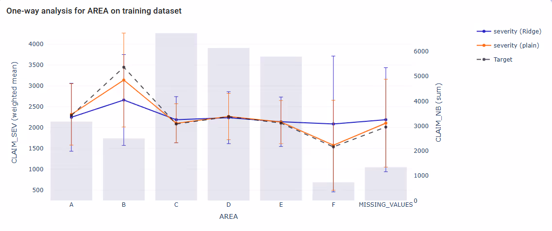
As we already know (link) simple GLMs and GAMs can’t really differentiate between low and high exposure data. No matter how many rows are in the table, the result will be more or less exposure weighted average of the target – main difference is the ability to derive meaningful statistical information from higher data volumes. The credibility methods are a solution here, and they are nothing new. The first ideas in the area date to a century ago (which lacked statistical rigour), to be then refined nearly sixty years later. The idea of blending simple predictions with expert knowledge may not be new, but has profound meaning and seems to be at heart of some modern actuarial modelling methods. It is especially useful in the area of commercial lines, where data is usually scarce. As it turns out, besides more classical formulations, there are also other methods which exhibit more or less implicit properties of weighting observation with expert knowledge. So let’s answer the following question: how much of credibility-like behaviour is in your price model? We will explore basics, extensions and more advanced modelling methods (in the order of increasing abstractions) to find it out.
Weighting with experience
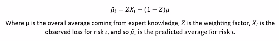
In the credibility approach we assume that each risk follows some distribution of losses and each claim is independent from the other. We observe only a sample from the distribution, and the true underlying loss distribution is unknown. At the core of the method there is the well-known formula:
The trick is to find a meaningful way to compute the Z factor. In the classical formulation of the Bühlmann-Straub it is calculated in the language of within/between-risk variance (𝐸𝑃𝑉&𝑉𝑀𝐻) and total risk exposure (in the earliest formulation there was the assumption on equal exposures, which was taken care of later). It is usually represented as:
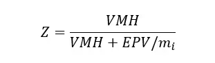
Where mi stands for total exposure for risk i. From the mathematical point of view it is clear that this kind of formula assigns higher Z values (closer to 1) to risks with larger total exposures, and lower (closer to 0) for risks with low exposure. This way we introduce a correction to the base model using additional piece of information, which may be external to the training data. The overall average may come from the dataset used for training and validation, but may as well come from publicly available market statistics. The remaining parts of the formula (𝐸𝑃𝑉&𝑉𝑀𝐻) are derived directly from the data in the language of means and variances. This way the weight is derived directly from the data and only the overall means are updated as expert judgement.
Going deeper
One of the strong parts of the classical formulation is the fact that it is distribution-free. The method uses only first and second moments, and these can be estimated based on data volume and volatility. However, if we take a step back and allow ourselves a bit of generality, we see the method is rooted in Bayesian statistics. Maybe not in the strict meaning of the word, but let’s take a closer look at it.
First, let’s remember the Bayes Theorem:

While working with a full Bayesian model we have to formally assume a prior distribution for each risk’s true loss parameter. Then it is updated according to Bayes theorem with observed data. The result is the posterior distribution of the parameter. The posterior expected loss will be a weighted average of the prior expectation and the sample mean – which is exactly the core statement in the credibility theory! It’s usually not exactly like it, however we can treat standard credibility formulas as approximations of special cases of Bayesian updating. It can be shown that the best linear unbiased predictor of the Bayesian result (optimised with respect to least squares) is actually the Bühlmann’s model (source).
Another link we can make here is the fact that the prior in Bayesian modelling represents (in our context) the actuary’s belief or the population’s characteristics. These do not need to come from the data. Then, as more data accumulate for a given risk, the influence of the prior diminishes and the posterior relies more on that risk’s actual experience – mirroring the idea that credibility increases with volume of data.
The Bayesian method has a very practical advantage which is probabilistic interpretation of uncertainty. The expert knowledge can be incorporated via prior distribution with higher complexity than simple overall mean. On the other hand, full Bayesian calculations are way more complex and require having an informative prior distribution. In practice, Bühlmann’s model is close enough to the Bayesian one.
Turning to linear models
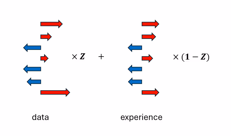
Blending
Anyway coming back to our daily actuarial life, we know it is GLM (or more generally GAM) framework that we use most often. As I mentioned at the very beginning – the basic formulation of linear models implicitly assumes full credibility for each segment. No matter how little data is available for the segment, the observed mean is not weighted towards anything more general. This can lead to an overfit to extreme values in sparse levels.
One way to improve a GLM using the credibility theory is to employ the core credibility formula with 𝑋𝑖 substituted for the trained model and adjust its predictions using a credibility complement weighted by exposure. The assumed relativity can be derived from, for example, a neighbouring coefficient or an all-other-cell average. This way the actuary does not have to resign from using GLMs at all and can base the adjustment on segments where the model lacks exposure. This targeted approach is often accepted by regulators, particularly when it ensures stability in sparse segments and smooths noisy estimates. However, it has some drawbacks – it requires manual adjustments, the more of them, the larger the model. So in itself it opens up possibilities for manual input errors. Of course, it also lead to lower overall model precision.
Looking for the idle
We often find ourselves in a situation, where the dataset used for model training contains variables, which clearly impact the target variable, but adding them as a model feature would be more of an issue than a solution. The best examples here are zip code or a vehicle make-model. Both are nominal variables with thousands of levels. For now let’s focus on geographical data, keeping in mind that geographical modelling is a broad topic in itself and this would not be a method typically used to deal with it. So let’s assume we have individual policies grouped by zip codes, which in turn belong to broader regions. It is quite clear that one zip code can be attributed to only one region, so the assumption on independence of features is broken here. Including both region and zip code as fixed effects in a GLM would cause collinearity and explode the model complexity. This would result with unreliable predictions, so we usually exclude zip code as a simple feature – it becomes a latent variable (meaning it has a clear impact on the prediction, but is not included as a feature).
This is an example of a hierarchical data structure (non-independence of features, clear groupings, etc.) and it requires a different approach. There already exists a general framework of Mixed Models, which are designed to deal with hierarchical data structures. There is also an extension of GLMs including mixing effects and it is called GLMM or Generalised Linear Mixed Model.
Keeping the example with region and zip code in mind, let’s think of it this way: what if, instead of training a model with both region and zip code as a fixed features, we could draw the “betas” for zip code from a distribution – a random effect, while keeping region as a fixed-effect feature?
Yes, it sounds weird, but let’s introduce such latent group-level factor as random effects, which are following some probability distribution (usually normal with mean 0 and unknown variance σ2u).
Now the central equation of the model becomes

Here β represents the fixed effects, u the random effects and Q is the random effect design matrix (think of it as a group selector, or one-hot-encoding of the latent variable). Next, according to the law of total probability, we integrate out u to obtain the marginal likelihood for MLE, and solve for fixed effects β and variance σ2u – note we’ve just reduced the full complexity of the zip code variable to a single variance parameter! Then, using Bayes' rule, we estimate the random effects u from the data. We arrive at the best linear unbiased predictor (or BLUP) of the true random effect u:

Now, it’s a matter of simple algebra, to reorganise the equations and arrive at:

or equivalently, at group level
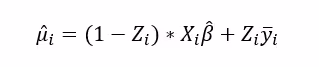
This is exactly what we are looking for – the core formula of the credibility method! An important closing note is that it’s not simply a blend of predictor for fixed effects with a credibility complement – β and σ2u are estimated jointly, so the two affect each other.
Smoothing
One of the fundamental weaknesses of GLMs, as mentioned earlier in this section, is the fact that a GLM does not inherently distinguish between segments with low and high exposure, which can lead to overfitting on extreme or less credible data. However, a variant of the model allows for correction – penalized GLMs.
Their story dates back to 1960s when Ridge regression was developed as a way to deal with singularity of design covariance matrix, which was caused by collinearity of model features. In unregularized case, betas are estimates as:
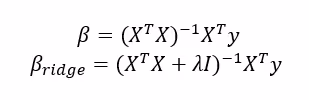
Where XTX is the design covariance matrix. Singularity here means that the design matrix cannot be inverted (or if the matrix is nearly singular, then it is numerically unstable). The idea was to add a regularisation term that improves the invertibility of the design matrix –– and lower model variance, at the cost of increased bias. It turns out this modifies ordinary least squares minimisation problem in such a way, that a penalty on the betas appears in the equation
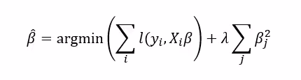
The positive penalty on the coefficients in the minimisation formula puts a negative pressure on the size of the betas. However, it keeps the collinearity in the model, although the coefficients are reduced close to zero. It was later improved with Lasso method to add absolute values of betas instead of squares
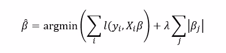
Due to the geometry of the reformulated problem, the solutions are more likely to be zero for some features, especially the collinear ones. And again – the nature of the penalty implies a reduction in coefficient absolute size. This is extremely important for segments with low exposure. As the number of policies in a segment increase, the laws of large numbers are at work and the resulting mean gains credibility. Consider claim severity model, where a segment contains a low number of high value claims, which yield a large coefficient. The result is a very high coefficient – not really credible, but the GLM has no way to “see” this. On the other hand when the Lasso penalty is applied, the optimization process shrinks large coefficients toward zero. In effect large betas are shrunk towards zero, which means the predictions for such segments are closer to the overall mean (the intercept, adjusted for the remaining features).
It should be clear by now, that the technique effectively weights observations toward the overall mean in segments with lower exposure. That’s again the core concept of the credibility theory, however here it remains implicit – the formula cannot be observed directly. Having said that, a GLM with Lasso might be a step in the right direction for commercial lines pricing, especially if GLM framework is already used. It’s a simple step to include credibility-like shrinkage in a data-driven way, without reliance on external parameters. On the other hand, the method introduces a systemic bias and lowers the explainability of the model coefficients. So it seems to be a nice first step towards credibility theory, however more explicit methods provide more clarity and allow more control over coefficients.
Seeing beyond
As we can see, the credibility theory extends beyond its explicit formulas and a credibility-like behaviour can also be observed in more complex models. In fact, a similar behaviour can be observed in Random Forests. So let’s remember they are an ensemble method, meaning the predictor consists of multiple base models—individual decision trees in this case. It has the following formula:
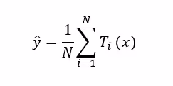
Where N is the number of trees, and each Ti(x) is a prediction of the i-th tree for input x. So we see it’s already an average of all predictions. A sufficiently large N is required for stable predictions. The optimal number depends on the dataset size: in personal lines with datasets exceeding a million rows, N should typically be greater than 1000; in commercial lines or with smaller datasets, N should be considered between 300 and 1000. And how is each tree constructed? In general they are created independently, in the same way. First a bootstrap sample (with replacement) is drawn from the data, then the columns are sampled (so not all features are used!), to finally compute a set of optimal splits (to minimise some kind of task-specific purity/quality measure) in the data.
Now, let’s return to the general example used throughout this blog post: a model with a segment that has low exposure but contains extreme values—let’s say this segment represents a small fraction of the total dataset. Each tree is trained on a bootstrap sample drawn with replacement, meaning some data points may be left out. On average, about 63.2% of unique observations appear in each sample (see the derivation e.g. here). A split occurs only if there is sufficient data to justify it; otherwise, a sparse segment is merged into a broader group.
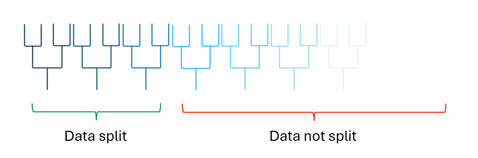
Some trees may recognise the segment in a split and produce estimates for it, but these estimates are based on a small number of observations, making them less reliable. Otherwise, the tree merges less frequent profiles with larger, more established groups. So a Random Forest exhibits weighting against some kind of overall mean along two axes: within-tree (sparse segments are often merged with larger groups when insufficient data is available to form a separate split) and between-trees (only a fraction of trees explicitly split the segment). In the last case we can write it as
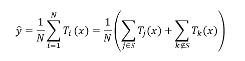
Where S is the set of indices for trees that created a separate split for the low-exposure segment. So the final prediction is implicitly weighted by the proportion of trees that recognize the segment in a split. To wrap it up, Random Forest seems to be a general machine learning technique with built-in two-dimensional credibility-like feature.
Just to mention other methods – there is already a novel approach that explicitly incorporates the credibility mechanism within neural networks using transformer architecture (transformers are at the heart of modern AIs, like ChatGPT). While neural networks traditionally struggle with tabular, structured data – common in insurance pricing – transformer-based architectures have the potential to improve performance in this area.
Credibility methods are a powerful way to balance actuarial rigor with data-driven pricing. How do you incorporate credibility in your models? Are there any specific challenges you face when blending expert judgement with predictive models? Would you like to learn more about how Quantee deals with low-credibility segments in commercial lines?
%20(2).avif)